Computers compress and decompress data all the time. Every webpage is compressed before being sent to your browser. Compression saves money, bandwidth and loading time. Lossy compression simplifies data and removes details whilst retaining the essential. For example, MP3 removes frequencies inaudible by most humans, and JPEG reduces details and colour information. On the other hand, lossless compression guarantees that the data will be the same as the original after decompression. How can you make something smaller without losing any details? Magic? The secret is to look for patterns, repetitions and predictability.

RLE

Run-length encoding (RLE) is one of the most straightforward lossless compression algorithms. The idea is simple: when you see a repeated symbol, compress it by storing the number of repetitions next to the symbol. A symbol could be a number, a letter or a bit (zero or one).

Consider an image file where we use capital letters to denote a pixel colour: WWWWWBBBWWBRRR (W is White, B is Black, R is Red…). Following the algorithm we can compress WWWWWBBBWWBRRR into: 5W3B2WB3R. By doing so, we saved four symbols. The compression ratio is 0.64 (9/14).

The algorithm is simple to code. Move forward and count any repetition of the same symbol.

def rle(data):
    encoding = []
    previous_symbol = None

    for symbol in data:
        if symbol != previous_symbol:
            if previous_symbol:
                encoding.append((count, previous_symbol))
            count = 1
            previous_symbol = symbol
        else:
            count += 1
    else:
        encoding.append((count, previous_symbol))

    return "".join(
        [f"{count}{symbol}" if count > 1 else f"{symbol}" for count, symbol in encoding]
    )

>>> rle('WWWWWBBBWWBRRR')
>>> '5W3B2WB3R'

RLE is a quick introduction to data compression. This algorithm works well with repetitions and patterns. Every compression technique has pros and cons and performs particularly well with one data type (e.g., photography, illustration, text).

Encoding

Let’s come back to data and remind ourselves about encoding. How are numbers and letters represented inside a computer?

Consider a limited set of symbols: the lower case alphabet and space.

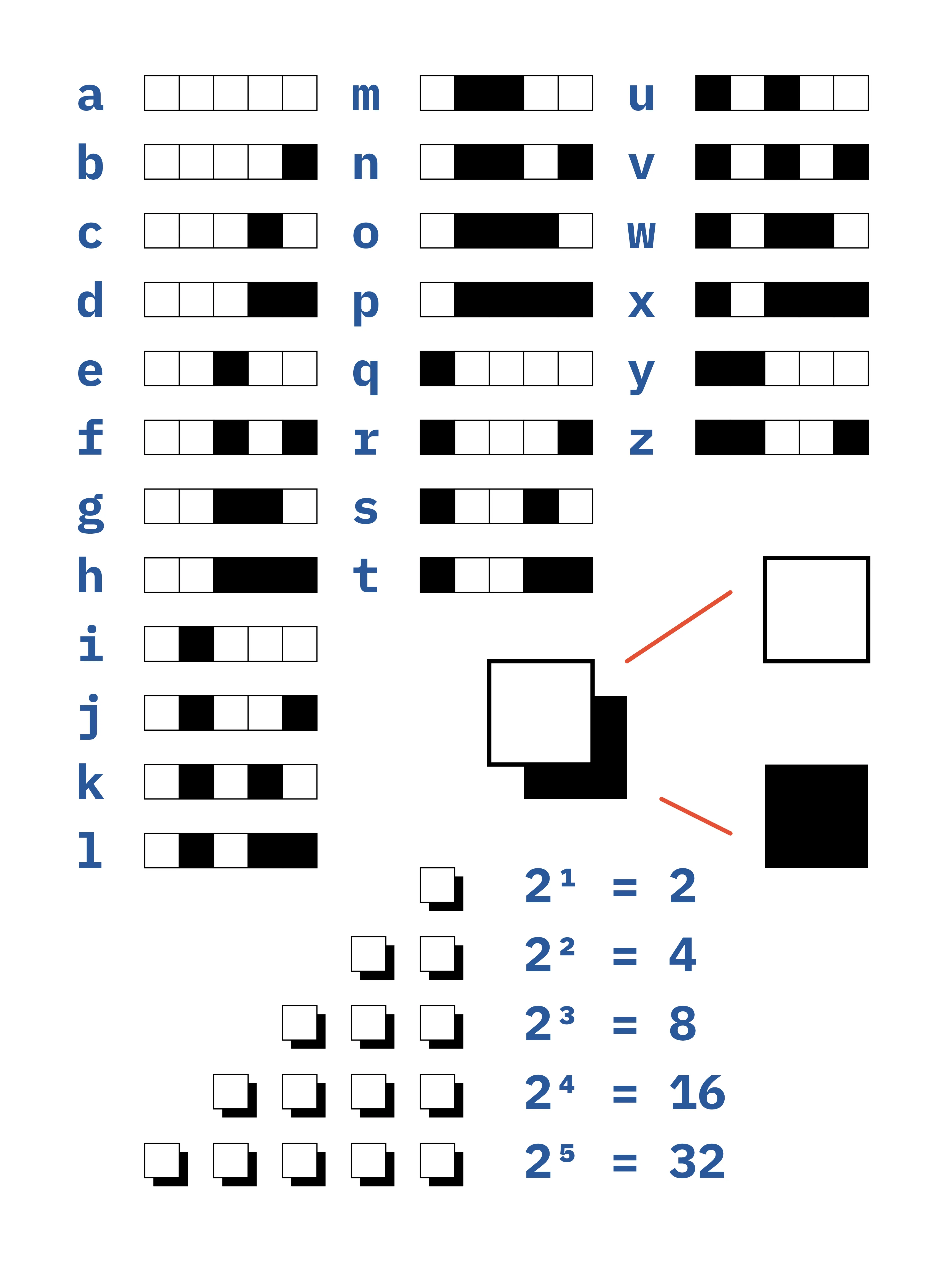
' ' 'a' 'b' 'c' … 'x' 'y' 'z'

With 27 symbols, we need at least 5 bits to represent one character (2^4 = 16 < 27 < 2^5 = 32).

Each symbol gets a unique binary code that a computer can process:

'a' 00000
'b' 00001
'c' 00010
'd' 00011
'e' 00100
…
'x' 10111
'y' 11000
'z' 11001
' ' 11010

This is a dictionary; each symbol maps to a unique binary code. Our toy encoding system is a subset of ASCII, which is a character encoding standard. The good thing about being a standard is that every computer understands ASCII encoded data. ASCII uses 8-bit codes. You might have heard of Unicode, which includes many more characters and emojis. It uses variably 8-bit, 16-bit or 32-bit codes.

If we were to represent the sentence “i ate an apple” with our encoding system; it would weigh 70 bits (14 symbols * 5 bits).

0100011010000001001100100110100000001101110100000001111011110101100100

Can we make this sentence weight even less by compressing it? We can’t use RLE as there are no repeating patterns.

What else could we do?

You might have noticed that we are using fixed-length codes. Fixed-length codes make decompression easy because we know how long each encoded symbol is. Indeed, we read the data in chunks of 8 bits.

Could we use variable-length codes to save space?

Symbols in our alphabet that appear the most often could have smaller code, whereas infrequent symbols could have longer code. However, variable-length code complicates things. Going through the compressed data, you won’t know where a symbol starts and ends. We could use a special marker to indicate the start and end of a symbol at the expense of extra space. There is another solution.

Huffman coding

Some symbols appear more often than others. What if we could use shorter codes to represent high-frequency symbols and longer codes for low-frequency symbols? One requirement is that the codes need to be unique. When reading the compressed data, we need a way to know when a symbol starts and ends.

Huffman devised an algorithm that exactly does that in a paper called “A Method for the Construction of Minimum-Redundancy Codes”. Given a set of symbols, the algorithm finds variable-length codes sorted by their respective usage frequency. To achieve that, it relies on a well-known data structure: the binary tree.

Binary Tree

A binary tree is a tree data structure where each node has two children. You insert new nodes by following the following rules:

• If the value of the new node is higher than the parent, go to the right
• If not, go to the left
• Add the new node when you can go right or left

A binary tree is great at keeping data sorted and maintaining a hierarchy. How does the Huffman algorithm use it?

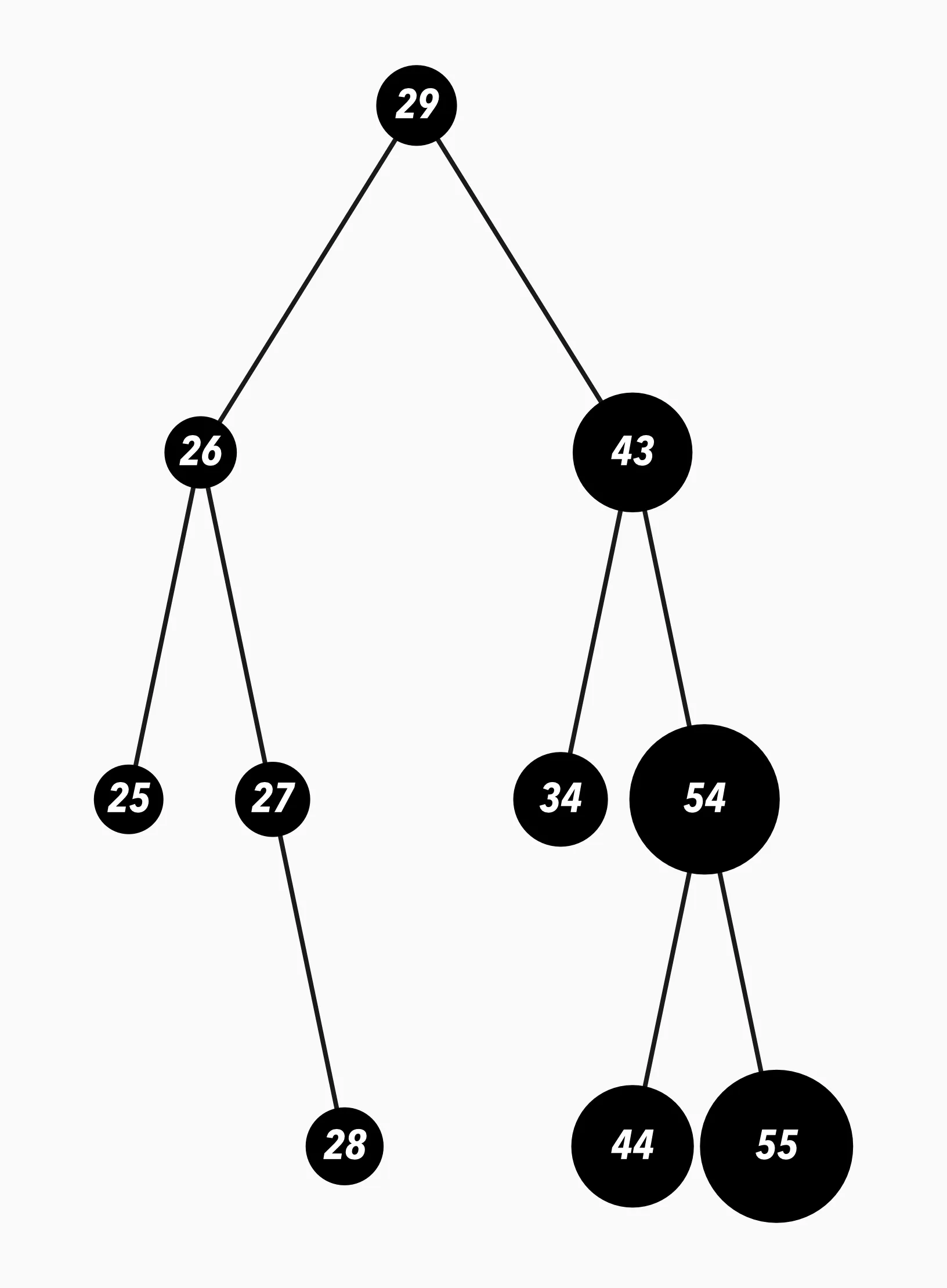
Binary tree created with the following values inserted in this order : 29, 26, 27, 43, 54, 25, 34, 28, 44, and 55.

Huffman algorithm

The algorithm is a bit complex but quite easy to follow step by step:

• Find the alphabet (all the symbols) of your data
• Sort symbols by frequency
• Insert symbols in a binary tree
• Read the binary tree to find out the unique code for each symbol

class Node(NamedTuple):
    frequency: int
    symbol: str
    left: Optional[Node]
    right: Optional[Node]

def huffman(data: str):
    counter = Counter(data)
    frequencies = counter.most_common()
    queue = []

    for symbol, freq in frequencies:
        heappush(queue, Node(freq, symbol, None, None))

    while len(queue) > 1:
        node_left = heappop(queue)
        node_right = heappop(queue)
        parent = Node(node_left[0] + node_right[0], "", node_left, node_right)
        heappush(queue, parent)

    tree_root = heappop(queue)

    return tree_root

First, we use a counter to count the occurrence of each symbol. We aim to place the most frequent symbols at the top of the tree. We start by adding all the symbols into a queue sorted by frequency (Python has a built-in implementation called heappush). The symbol with the highest frequency is a the start of the queue, and the symbol with the lowest frequency is at the end of the queue. The queue helps us track which symbol we need to insert next in the tree. Our binary tree is created with the help of the Node class. Each Node instance has a left and a right child.

When we are done building our binary tree, we can proceed with reading it to find the unique short codes for each of our symbols.

def dfs(tree, code='', dic={}):
    if not tree:
        return
    _, symbol, left, right = tree
    if symbol:
        dic[symbol] = code
    dfs(left, code + '0')
    dfs(right, code + '1')
    return dic

We start at the root of the tree. When we go left, we record a 0. When we go right, we record a 1. We continue until we end on a node with a symbol. The 0 and 1 encountered on the way make up the binary code of this symbol! This way of reading a binary tree is called a depth-first search. Here we use a recursive algorithm.

>>> tree = huffman('i ate an apple')
>>> codes = dfs(tree)
>>> print(codes)
>>> {' ': '00', 'a': '01', 'i': '1000', 'l': '1001', 'n': '1010', 't': '1011', 'e': '110', 'p': '111'}

We built our dictionary of unique binary codes. Notice how space and a are the most used symbols in our data; they are assigned the shortest codes.

Now that we have our dictionary where each possible symbol translates into a unique binary code, we can easily compress our data.

def huffman_compress(data, code_map=None):
    if not code_map:
        tree, _ = huffman(data)
        code_map = dfs(tree)
    return "".join([code_map[char] for char in data])

Remember the sentence we were trying to compress: “i ate an apple”.

In our toy encoding system, it weighed 70 bits (14 symbols * 5 bits).

Let’s compress it:

>>> huffman_compress('i ate an apple')
>>> 1000000110111100001101000011111111001110

The binary representation of the compression is 1000000110111100001101000011111111001110, which weight 40 bits.

By using variable-length codes, we went from 70 bits to 40 bits! Our compression ratio is a bit less than half. But this is without including the weight of the dictionary necessary for uncompressing it. This is extra data. You might find in some situations that the resulting compressed data plus the dictionary is bigger than the original file. It is not worth compressing such a small sentence, but with a longer one, the compression will be such that including the weight of the dictionary will be negligible.

Of course, you don’t need to build a dictionary every time. For example, you could reuse the English language dictionary for text written in English. This dictionary could be created by counting letter frequencies in thousands of books written in English. In this example, we used the frequency of the letters in the sentence we wanted to compress. In practice, we would use a different probability model. Instead of letters, we could have used words or fragments of words. Imagine using a short code for “the”, a popular determiner.

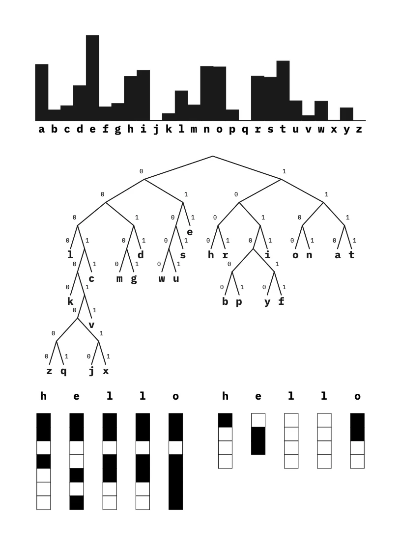
Compressing “hello” with variable coding. The probability model is built on the letters frequencies in The Waste Land by T.S. Eliot.

Shannon’s entropy

Could we compress our phrase “i ate an apple” even further? How do we know if we did our best?

Shannon’s entropy is a measure of information in data. It links probabilities with information.

The formula to calculate Shannon’s entropy is relatively short. It takes into input the probabilities of each symbol or event.

from math import log2

def entropy(probabilities: list[float]) -> float:
    return -sum([p * log2(p) for p in probabilities])

Let’s understand how it works by using a simple example; a coin.

>>> entropy([0.5, 0.5])
>>> 1.0

The entropy of a fair coin is 1.0. There is a fifty-fifty chance that you will land on a head or a tail. Shannon’s entropy tells us we need a least 1 bit to describe the results of a coin toss.

The entropy of a rigged coin (90% chance of getting a tail) is 0.46. We need less than a bit to describe the result of a toss. This is because most of the time, we know the answer.

>>> entropy([0.1, 0.9])
>>> 0.4689955935892812

When is entropy equal to zero? It’s when there is absolute certainty. A tricked coin that always lands on heads has zero entropy.

>>> entropy([0.0001, 0.9999])
>>> 0.0014730335283281598

Those examples show us how Shannon’s entropy measures randomness in data. Entropy helps answer a question: how much information is in a message? A rigged coin has low entropy and does not convey much information; we always know the result of a toss.

Measuring entropy has many applications. For example, entropy helps decides whether your password is strong enough. A password made of random letters is stronger than a password that can be easily guessed or that display a pattern. The higher the entropy of your password, the harder it is to break ¹.

If we calculate the entropy of our sentence “i ate an apple” we get the number: 2.81.

>>> probs = {'i': 0.07, ' ': 0.21, 'a': 0.21, 't': 0.07, 'e': 0.14, 'n': 0.07, 'p': 0.14, 'l': 0.07}
>>> entropy(probs.values())
>>> 2.814086992059893

This tells us that, in theory, we need a minimum of 2.8 bits to represent this sentence in binary. Therefore, the minimum theoretical weight of this sentence in binary is 14 * 2.81 = 39.34 bits. Remember the previous results; we managed to compress this sentence from 70 bits to 40 bits which is very close to the theoretical limit. Our compression scheme was effective!

Entropy and compression

We discovered that to compress data, we need repetitions and patterns. Entropy being a measure of randomness, we can intuitively say that:

• A low entropy data will compress well
• A high entropy data will not compress well

An image with random pixels will not compress well. An image displaying a pattern will compress well.

The entropy of a given sequence of symbols gives us a lower bound on the average number of bits required to encode the symbols. Entropy will tell you, in theory, how much you can compress a given data. Not every compression algorithms are equal and will let you compress to that theoretical limit.

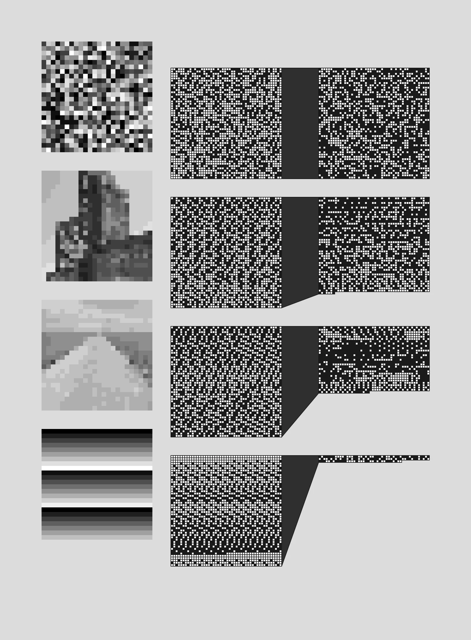
• Random pixels don’t compress.
• Pictures with a skewed distribution of pixel values compress well.
• The last image is compressed by RLE first and then Huffman coded.

Conclusion

You compress data essentially by looking for repeated patterns and predictability. We studied two basic compression algorithms that led us to talk about Shannon’s information theory and entropy. To continue, LZW is another interesting lossless compression algorithm. And there is more to learn; lossy compression algorithms are even more complex and fascinating.

Epilogue

Can you compress compressed data? Compression increases the entropy of data. A highly compressed data has a high entropy similar to a random source. This is because compression removes redundancy, repetitions and patterns. So no, zipping a zip file will never make the data smaller.

Footnotes

1. XKCD comic “Password Strength” ↩