
Projects, tasks, odds and the casino
No one ever finishes a project on time! Life gets in the way. Like a casino, life is the house and is consistently winning. Still, when we estimate a project, we pretend we have everything under control. What can we do to have a better hand? Is there a better way to model uncertainty and define more reliable estimates?
Task breakdowns
We embark on a project to build a website with a landing page and a contact form.
The first step is to consult our experts and write down some tasks:
- ”We need a copywriter”;
- ”We need to find an API to send emails”;
- ”Coding the landing page”;
- ”Designing the landing page”;
- etc…
Then, our experts decide in what order things should happen and how long each task should take. Finally, we sum up the task duration and add a contingency for the odd spoke in the wheel. Job done. The stakeholders now know when their project will end and how long it will take.
How did our experts come up with the estimations? Usually, we would do an estimation session using an Agile tool like Planning Poker. It’s a popular technique for getting numbers from a team in a playful way. Each participant has a deck of cards with numbers (e.g. 1, 2, 3, 5, 8…). Participants will draw a card from the deck and reveal their estimate when asked. When the numbers drawn are widely different, the team must discuss or postpone voting because it shows that the task is ambiguous. A solution is to do more research or split the task further, with the aim getting a consensus on the number.
In a Planning Poker1 session, you will often see individuals with a strong voice and others who will go with the majority. A junior colleague might be too optimistic compared to a senior. One could be overconfident, and the other could be underconfident. Another problem is that we get a fixed number out of the session. The information about uncertainty or level of confidence is lost in the averaging exercise. Also, estimating task by task doesn’t capture the interdependence of tasks and what effect one has on the other.
But what could we use instead of a fixed estimate? A probability distribution.
PERT
PERT stands for Program Evaluation and Review Technique. It’s a project management tool invented by the United States Navy in 1958. PERT uses a probability distribution to represent the duration of tasks and the project. Another aspect of PERT is using a graph or network to represent task dependencies. Let’s see how it works!
Instead of one estimate per task, we ask our team members for three numbers:
- Their pessimistic guess (worst-case scenario);
- Their likely or probable time needed to complete the task;
- And finally, their optimistic guess. If everything went right, how long would it take?
We call this a three-point estimate. Each activity has a weighted average duration that can range from an optimistic time to a pessimistic time.
One way to do a three-point estimate with Planning-Poker is to do the following:
- Take the lowest value of the pessimistic guesses;
- Take the highest value of the optimistic guesses;
- Get the average value of the likely guesses or agree on one by consensus.
Back to our project — our experts gave us their three-point estimate for each task, which we compiled in this table.
| Task code | Title | Predecesors | Likely | Optimistic | Pessimist | ||
|---|---|---|---|---|---|---|---|
| A | Setup | 16 | 14 | 20 | 16,33 | 1,00 | |
| B | Email API | 6 | 5 | 8 | 6,17 | 0,25 | |
| C | Research | 10 | 9 | 14 | 10,50 | 0,69 | |
| D | Design landing | C | 10 | 9 | 13 | 10,33 | 0,44 |
| E | Implement landing | A, D | 10 | 8 | 12 | 10,00 | 0,44 |
| F | Design form | C | 6 | 4 | 9 | 6,17 | 0.69 |
| G | Implement form | B, F | 6 | 5 | 8 | 6,17 | 0,25 |
| H | Editorial | C | 16 | 15 | 19 | 16,33 | 0,44 |
| I | Add content to CMS | E, G, H | 3 | 2 | 4 | 3,00 | 0,11 |
| J | Setup & deploy | I | 2 | 2 | 4 | 2,33 | 0,11 |
PERT distribution
Using a three-point estimate, we removed the need to discuss, up-vote or down-vote, what duration is wrong or right. We captured the range of opinions and colleagues’ uncertainty.
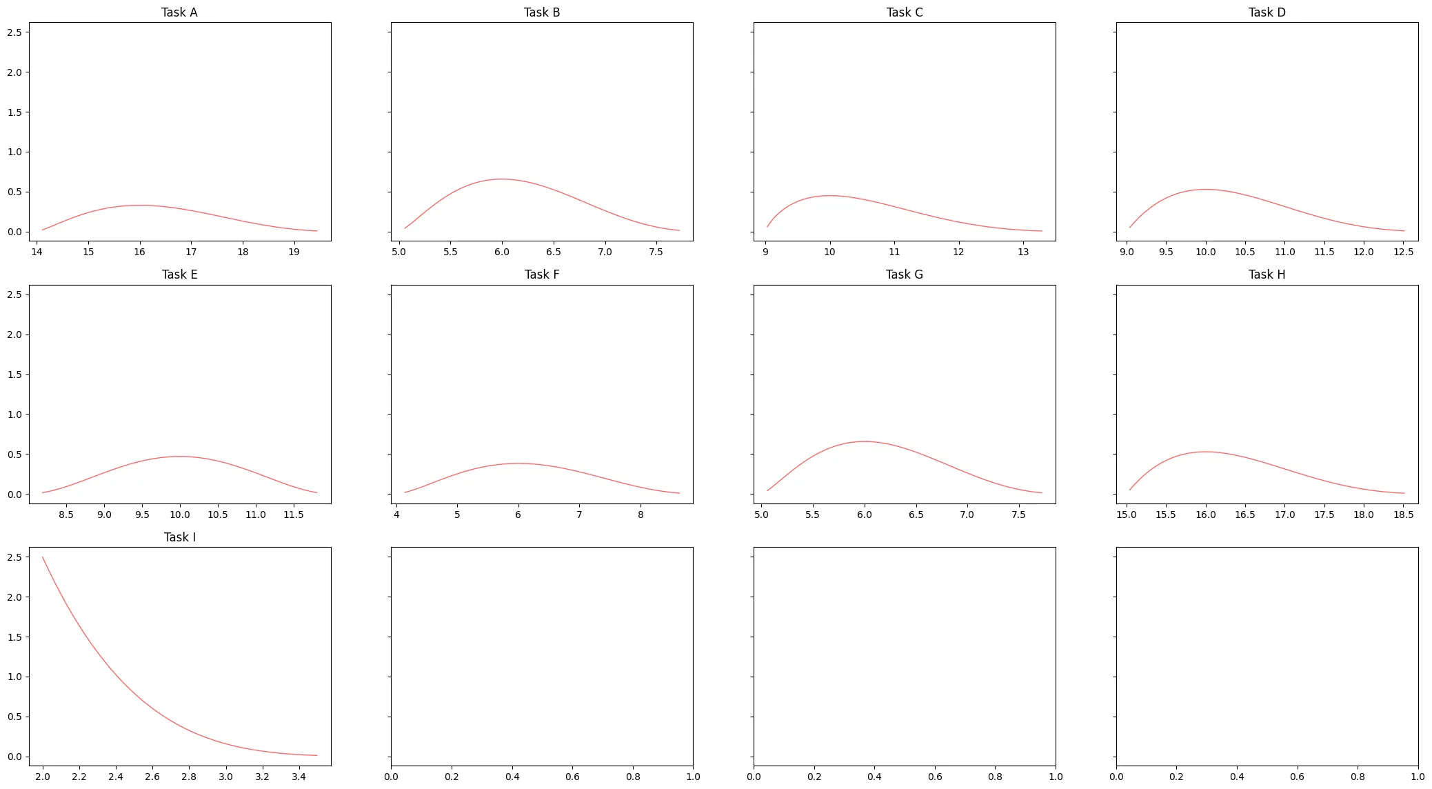
PERT represent this range by using the PERT probability distribution2, to capture the range of a task duration. The distribution looks like a bell curve that peeks around, but not precisely, at the likely guess and tails of the pessimist and optimist values.
Plotting the distribution of each task gives us an excellent visual indication of the risk associated with them. A curve with a high peak denotes certainty (e.g. task B), whereas a flat curve shows uncertainty on how long the task will take (e.g. task F).
We can calculate the expected duration of a task by computing the mean of the distribution defined by the three-point estimate. Note that the likely value of the estimate is not the mean. The mean of the distribution is defined as the weighted average of the minimum, most likely and maximum values that the variable may take, with four times the weight applied to the most probable value.
The variance is defined as follows:
The standard deviation (σ) calculation assumes that a beta distribution’s standard deviation is approximately one-sixth of its range.
For every task, we calculate its expected duration
| Task code | Title | Predecesors | Likely | Optimistic | Pessimist | ||
|---|---|---|---|---|---|---|---|
| A | Setup | 16 | 14 | 20 | 16,33 | 1,00 | |
| B | Email API | 6 | 5 | 8 | 6,17 | 0,25 | |
| C | Research | 10 | 9 | 14 | 10,50 | 0,69 | |
| D | Design landing | C | 10 | 9 | 13 | 10,33 | 0,44 |
| E | Implement landing | A, D | 10 | 8 | 12 | 10,00 | 0,44 |
| F | Design form | C | 6 | 4 | 9 | 6,17 | 0.69 |
| G | Implement form | B, F | 6 | 5 | 8 | 6,17 | 0,25 |
| H | Editorial | C | 16 | 15 | 19 | 16,33 | 0,44 |
| I | Add content to CMS | E, G, H | 3 | 2 | 4 | 3,00 | 0,11 |
| J | Setup & deploy | I | 2 | 2 | 4 | 2,33 | 0,11 |
PERT network
Now that we have the distribution mean for each task, we can draw the PERT diagram.
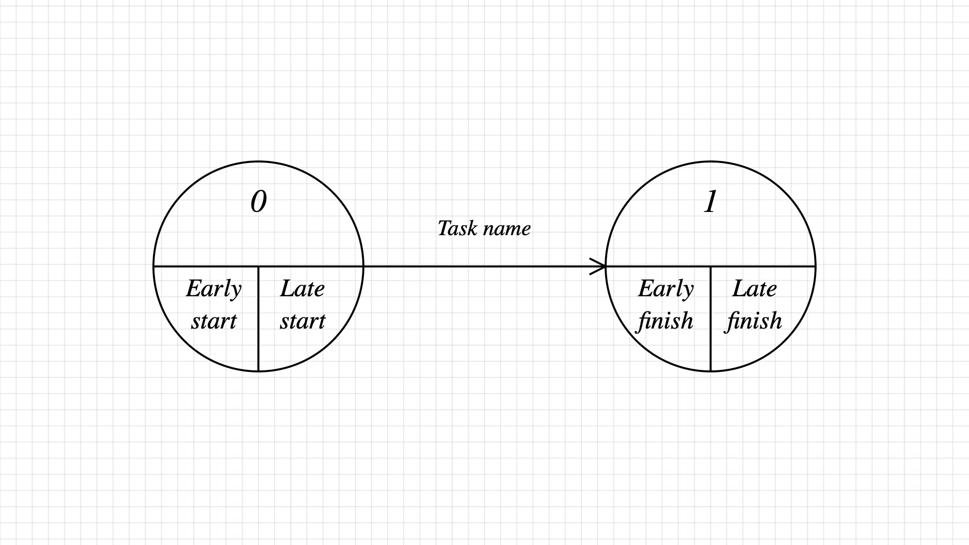
A PERT diagram is a graph where links represent tasks, and nodes represent a task’s start and end time.
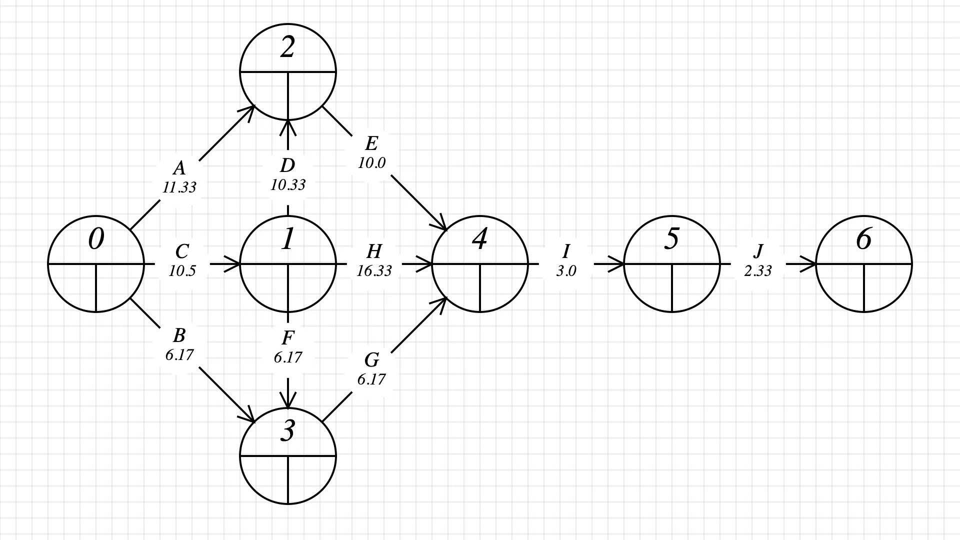
By connecting nodes, we represent dependencies in the project. With trial and error and a few iterations on paper, this is how I translated the tasks and dependencies into a PERT network. The graph displays dependencies; for example, J depends on I, and I depends on E, H, and G.
The node’s early start/finish and late start/finish are empty – let’s fill them in.
Step 2: fill in every node’s early start by adding the task durations. This is done by going from the first task to the last task in the graph. Pick the biggest early start/finish value for each node.
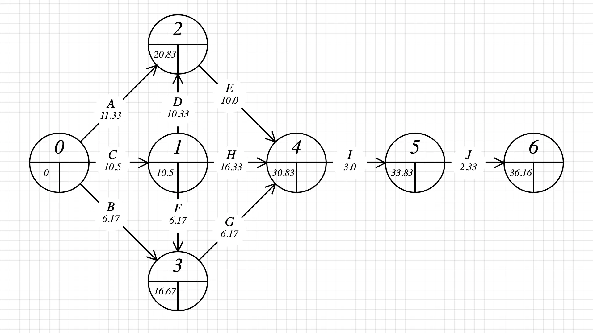
Step 3: fill in the late start/finish values. This is done by going from the last to the first task in the graph and subtracting durations. Pick the biggest late start/finish value for each node.
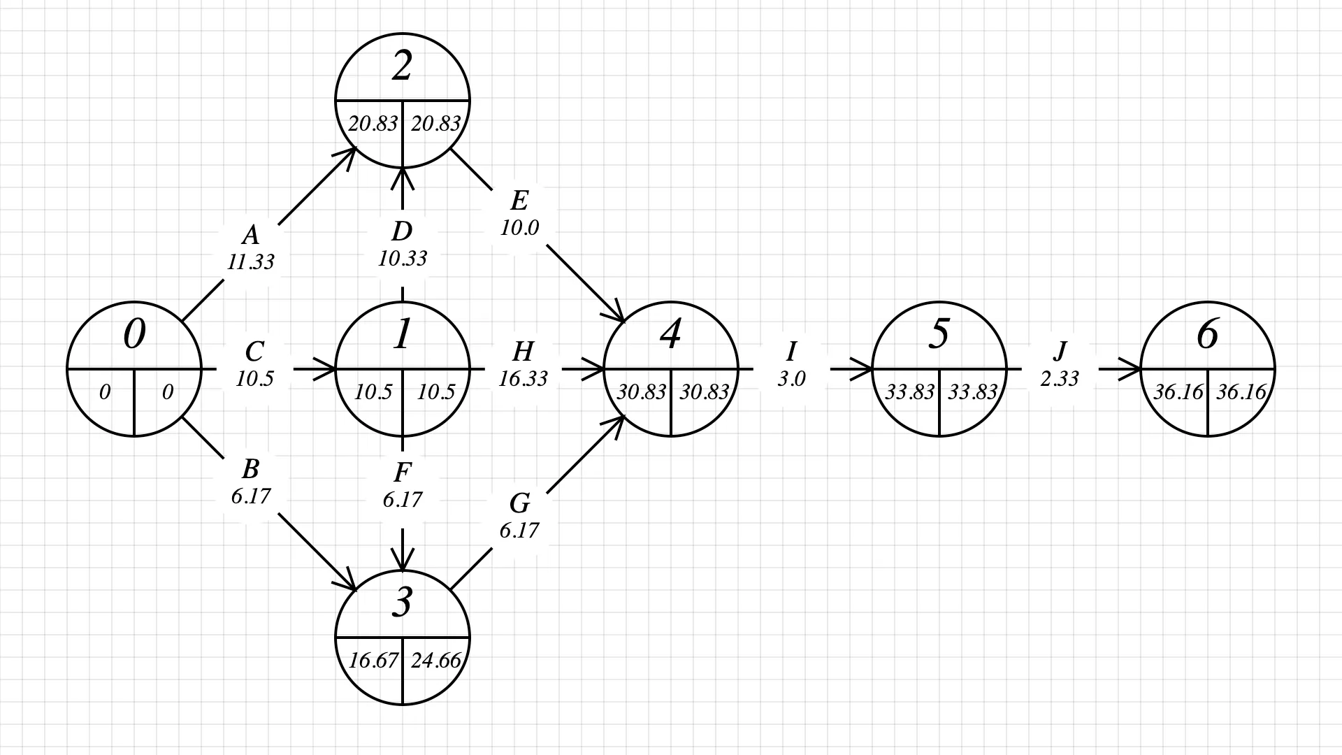
At the end of this step, we find our answer! The project can be completed in 37 days (we round 36.16).
Step 4: find the critical path.
Critical Path
PERT and the CPM (Critical path method) help identify tasks that require attention and focus if we want to finish the project on time. The critical path is the series of tasks that must be finished on time for the entire project to finish on schedule.
Tasks with the same starting and ending value will likely be on the critical path. Let’s study what’s going from node 2 to node 4. Node 2 ends at 20.83, and node 4 starts at 30.83, but task E takes 10.0 days. There is no wiggle time or slack. If we want to be on time, we need to stick to 10 days and no more. Any activities with zero slack are on the critical path.
By repeating this process for every transition between tasks, we find the critical path shown in red below:
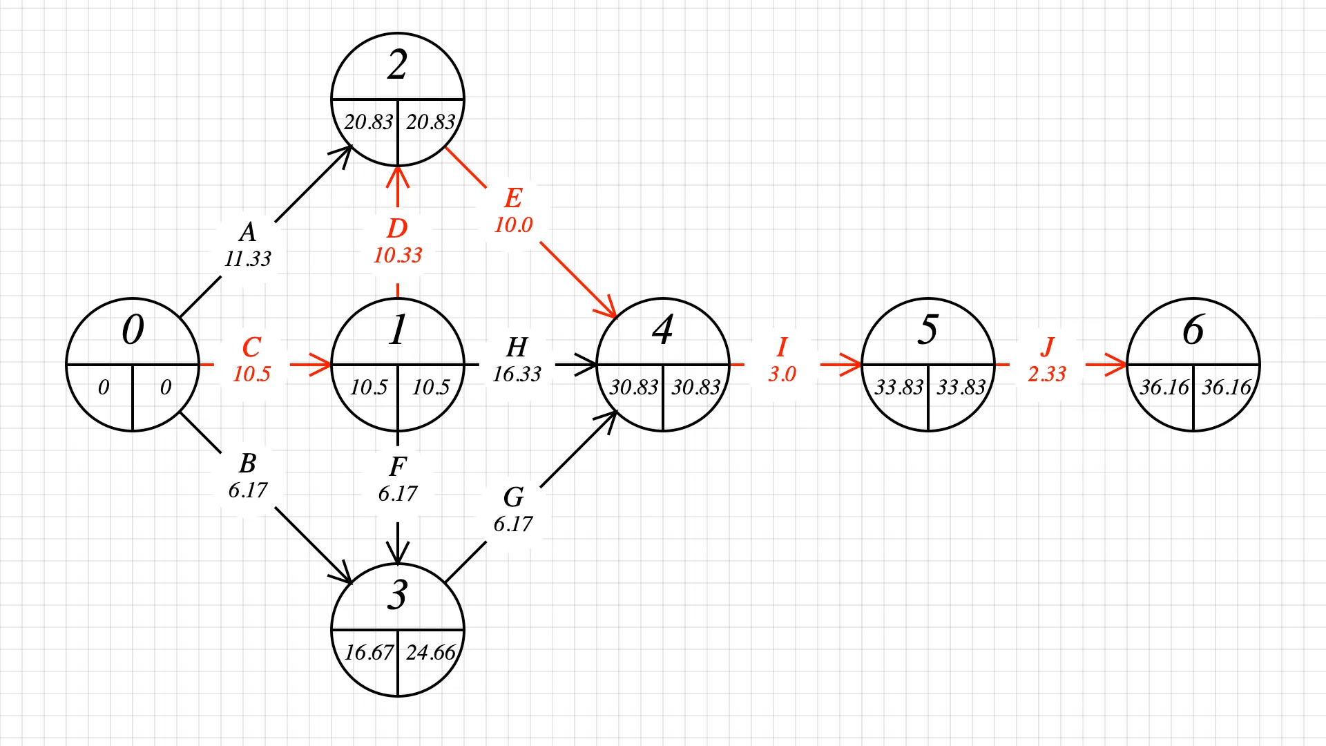
Any time lost on one of the activities C, D, E, I, or J will delay the project’s completion. The other activities have slack.
Note that the tasks on the critical path define the total project duration:
- The project’s mean duration
is the sum of the critical path’s tasks mean duration. - The variance of the project
is the sum of the critical path’s tasks variance. This also gives us the standard deviation.
We have the mean duration of the project
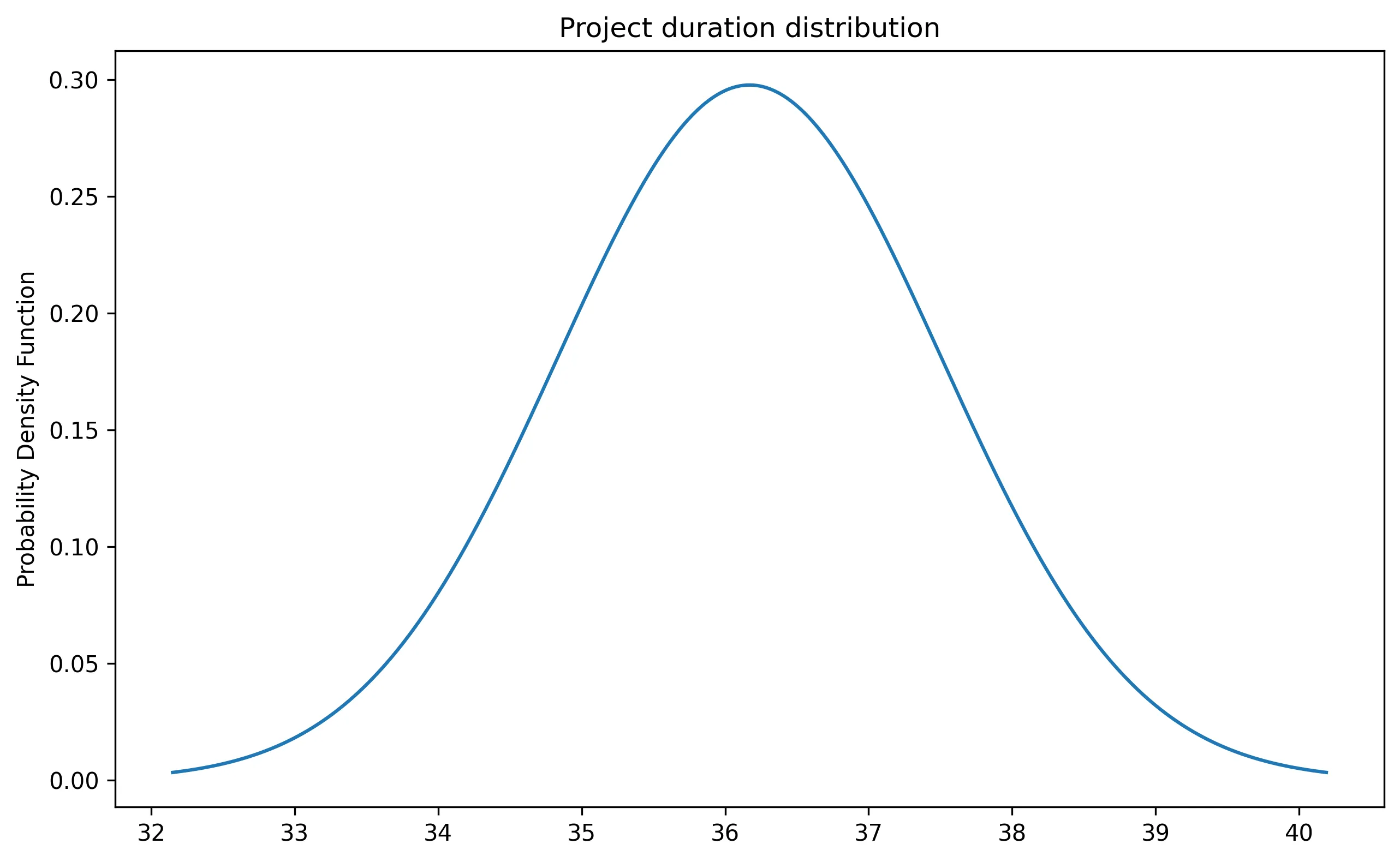
PERT assumes that the duration of each activity is a random variable with known mean and standard variation and derives a probability distribution for the project completion time.
- The duration of an activity is a random variable with a PERT distribution.
- The durations of the activities are statistically independent.
In its elegant simplicity, the Central Limit Theorem states that the sum or average of a large number of independent and identically distributed random variables approaches a normal distribution, regardless of the original distribution of the variables.
An example? Let’s say we have a classroom with a hundred students; we randomly sample thirty and ask about their body height. The distribution of the sample will go towards a normal distribution with a mean equal to the classroom average height! It’s spooky. Note that the sample size matters — the theorem only works if the sample is big enough.
Back to our project, the duration of each task is our population, and we are sampling the tasks on the critical path. The Central Limit Theorem lets us define the duration distribution of the project — a normal distribution with a mean of 36.17 days and a standard deviation of 1.34.
Applications
Equipped with the project’s duration distribution, we can answer some questions about the delivery.
What is the chance of meeting the deadline?
Our client is ready to sign a 37 days contract. Can we deliver on time?
We will need the project’s Normal distribution and cumulative distribution function (CDF) to answer this question. With Python, we can create an instance with the known mean and standard deviation.
A Cumulative Distribution Function (CDF) is a mathematical function that describes the probability that a random variable takes on a value less than or equal to a given point, providing a complete picture of the variable’s probability distribution.
from statistics, import NormalDist
nd = NormalDist(36.17, 1.34)
nd.cdf(37)
The result is:
0.73242827380114This means that the probability of finishing the project in less than 37 days is 73%. We are 27% likely to be late.
What is the chance of meeting the deadline within a range?
The client would like to know the probability of finishing the project between 37 and 32 days.
from statistics, import NormalDist
nd = NormalDist(36.17, 1.34)
nd.cdf(37) - nd.cdf(32))
The result is:
0.7312452320167355This means the probability of finishing the project between 32 and 37 days is 73%. In other words, the likelihood of finishing the project within a week of the deadline (37 - 32 = 5 days) is 73%.
What would be the duration that would meet a given risk?
The client doesn’t want any risk because of their planning and requirements. Of course, a 0% risk is impossible, so they are willing to have a 5% risk of being late. This translates into a 95% chance of finishing on time.
For that question, we need to use the inverse of the cumulative distribution function, which takes for input a probability.
from statistics import NormalDist
nd = NormalDist(36.17, 1.34)
nd.inv_cdf(0.95)
The result is:
38.37410386011497To have a chance of finishing the project on time with a 5% risk, we should sign a contract for 39 days instead of 37 days. Our client now knows when is best to launch their product.
Finding the probability distribution of the project helped us answer some interesting questions about the project and the risk associated with schedule.
With Monte Carlo method
Another technique3 at our disposal is to use a Monte Carlo simulation with PERT to get more accurate estimates.
How does a Monte Carlo simulation work?
Let’s say we want to find out if a coin is fair. The easiest way to do this is to toss the coin a significant amount of time. The probability of heads and tails will converge to a number that will tell us if the coin is fair. This is a simple Monte Carlo experiment.
Another example?
We can estimate 𝜋 by dropping random points within a square and calculating the proportion of points within an inscribed circle. Read this article for many more examples.
Back to our project!
Each task duration follows a PERT distribution that we can sample. For each simulation, we will draw a random duration for each task in the project. Each sampling gives us the total duration of the project.
How many simulations should we run? Remember, we rely on the Central Limit Theorem and need a large sample size. As I’m not a mathematician, I would say the more, the better, but a thousand sounds reasonable for this project.
Note that you could simulate with various distributions. For example, you could pick a distribution that is more skewed towards the pessimistic duration of a task because your team is very junior.
After running the simulations on this project, we find out:
The project mean duration is 33.86643 days with a standard deviation of 1.5215022363112058.
The advantage of this method is that we can find more than one critical path. The simulation found a second critical path: A, E, I, J (the original path was C, D, E, I, J). This tells us that in some situations, we need to pay more attention to other tasks than the ones in the original critical path.
Is it worth it?
Projects are not deterministic processes; they are stochastic. The only way to know how long a project will take is to do it. Having done a similar project in the past can help narrow down the guesses. The beauty of PERT and Monte Carlo is that they let us define a range of possible task durations and try various combinations to see how they impact the project’s completion.
The adage says ”garbage in, garbage out”. The numbers will be inaccurate if the three-point estimates are incorrect or need more research. That’s why we want to be thorough in our research and how we define tasks.
The most important estimation resource you have is the people around you. They can see things that you don’t. They can help you estimate your tasks more accurately than you can estimate them on your own. — Robert C. Martin in The Clean Coder
Remember that the map is not the territory. However, it’s better to have a map, even a wrong one, than nothing. The important thing is to update it in light of new information or when the project’s requirements change during implementation. A PERT network can help update estimates and evaluate the cost of changes. For example, if a change is not affecting the critical path, we should be okay with proceeding with it. The critical path helps us focus and pay attention to the tasks more likely to create delays.
In preparing for battle I have always found that plans are useless, but planning is indispensable. — Dwight D. Eisenhower
Using the three-point estimates (optimistic, most likely, pessimistic) represents a simplified way of assigning a probability distributions to each activity. In another follow-up article, I will describe another method to obtain the probability distribution of a task using random sampling (Monte Carlo methods).